Is V2 actually better? Paired testing for LLM releases

Say we run a RAG chatbot for an online pharmacy. V1 is in production. V2 only changes the system prompt. A few colleagues tried V2 by hand, and they think the answers are better.

Maybe they are right. But a handful of manual checks can’t separate a 6-point improvement from luck, and it says nothing about whether V2 got worse on the questions that matter most. Before V2 replaces V1, I want to know if we are testing the right questions, if the gain is bigger than sampling noise, and if it hides a regression we can’t accept.

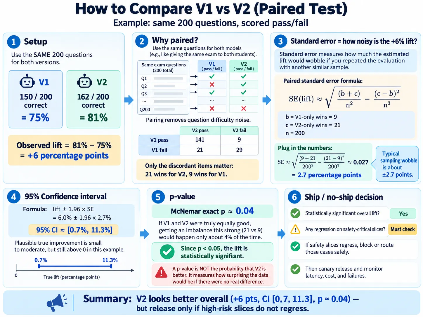
I’ll use one example for the whole post: V1 and V2 answer the same 200 questions, and each answer is scored pass or fail. The infographic is the short version.

Dataset coverage vs. standard error

The first instinct is to ask whether the evaluation set is big enough. But “big enough” mixes two different questions.

One is representativeness: do the evaluation questions look like real traffic? If 80% of production queries are about shipping and 1% are about drug interactions, a set with only shipping questions tells you nothing about safety. Adding more shipping questions doesn’t fix that.

The other is standard error: how much would the measured pass rate move if we ran the evaluation again on a different random set of questions?

More data only helps with the second one. With 10,000 badly sampled questions, you get a very precise estimate of the wrong thing. So I’d sort out coverage first (production queries, past failures, and extra high-risk cases on purpose), and only then ask how many questions we need.

Independence matters too. If 400 questions are paraphrases of 10 originals, you have something closer to 10 observations than 400. All the formulas below assume each question is its own draw.

A small naming thing, because the two terms get mixed up a lot. A paired evaluation means both versions answer the same questions. A pairwise preference evaluation means a human or a judge model picks the better of two answers. You can do both at once, but they are different designs. This post is about the paired one.

Standard error of one pass rate

Say a model really passes 80% of questions in the target population. Sample 100 questions and you might see 78 passes. Sample another 100 and you might see 83. The model is the same in both cases; the difference comes from which questions were drawn.

Standard error (SE) is the typical size of that wobble. For pass/fail scores:

\[\operatorname{SE}(\hat{p}) = \sqrt{\frac{\hat{p}(1-\hat{p})}{n}}\]

$\hat{p}$ is the observed pass rate and $n$ is the number of questions. For $\hat{p}=0.8$ and $n=100$:

\[\operatorname{SE} = \sqrt{\frac{0.8 \times 0.2}{100}} = \sqrt{0.0016} = 0.04\]

So about 4 percentage points. With 400 questions it goes down to 2.

We used four times more questions and the uncertainty only halved. That’s because

\[\operatorname{SE} \propto \frac{1}{\sqrt{n}}\]

Doubling $n$ multiplies SE by about 0.71. To get SE down to a quarter, you need sixteen times the questions. Labeling gets expensive fast, so I’d rather decide the target before collecting anything.

How many questions?

To answer “why 200 and not 500?”, you first have to say what you’re trying to do. Usually it’s one of these:

• estimate one version’s pass rate to some precision, or
• detect an improvement of V2 over V1 of at least some size.

For a release decision it’s the second. Say V1 passes about 75%, and the team agrees anything under 6 points isn’t worth shipping. Then fix these before running anything:

• minimum detectable effect $\delta = 0.06$
• significance level $\alpha = 0.05$
• power $1-\beta = 0.80$
• expected discordance rate $\psi = 0.15$, i.e. the share of questions where V1 and V2 get different results

The discordance rate is there because of the pairing. If both versions pass a question, or both fail it, that question says nothing about which one is better. Only the disagreements count. Two prompts on the same RAG system usually agree on most questions, and fewer disagreements means less noise in the difference.

A rough formula for paired pass/fail data:

\[n \approx \frac{\left(z_{1-\alpha/2} + z_{1-\beta}\right)^2 \psi}{\delta^2}\]

With $z_{0.975} \approx 1.96$ and $z_{0.80} \approx 0.84$:

\[n \approx \frac{(1.96 + 0.84)^2 \times 0.15}{0.06^2} \approx 327\]

So I’d plan for around 330 paired questions. Treat this as a planning number. An exact power calculation can come out different, and safety-critical slices need their own sample, usually a bigger one.

80% power means that if the true improvement really is 6 points (and the assumptions hold), the test catches it in about 80% of repeated experiments. It doesn’t mean there’s an 80% chance V2 is better. Power describes the test procedure under a specific alternative, and says nothing directly about the model.

The example below only has 200 questions. I ran a quick simulation of the exact McNemar test under the same assumptions: with 200 questions it detects a real 6-point gain only about 52% of the time. With 327 it’s about 78% (the exact test is a bit conservative). So the example is underpowered. A significant result is still a result, but if it had come out non-significant, we’d have learned very little.

Running both versions on the same questions

V1 passes 150 of 200 (75%). V2 passes 162 (81%). The observed lift:

\[\hat{\Delta} = 0.81 - 0.75 = 0.06\]

For a paired analysis you need the per-question results, not just the two totals:

	V2 passes	V2 fails
V1 passes	141	9
V1 fails	21	29

So 141 questions pass on both, 29 fail on both, $b = 9$ pass only on V1, and $c = 21$ pass only on V2.

Only 30 questions changed. The net gain is 12 questions:

\[\hat{\Delta} = \frac{c - b}{n} = \frac{21 - 9}{200} = 0.06\]

Same 6 points as before, but now you can see where they came from. V2 fixed 21 questions and broke 9. I’d read those 9 one by one before computing anything else. That’s usually where you learn what the new prompt actually changed.

Standard error of the difference

Give each question a score of $+1$ if only V2 passes, $-1$ if only V1 passes, and $0$ otherwise. The average of these scores is $\hat{\Delta}$. Both versions answered the same questions, so their results are correlated, and the SE has to account for that. You can’t treat the two pass rates as independent samples.

For paired pass/fail data:

\[\operatorname{SE}(\hat{\Delta}) \approx \sqrt{\frac{b + c}{n^2} - \frac{(c - b)^2}{n^3}}\]

With $b=9$, $c=21$, $n=200$:

\[\operatorname{SE} \approx \sqrt{\frac{30}{200^2} - \frac{12^2}{200^3}} = \sqrt{0.00075 - 0.000018} \approx 0.0271\]

That’s about 2.7 percentage points.

If you ignore the pairing and use the usual formula for two independent samples, you get:

\[\sqrt{\frac{0.75 \times 0.25}{200} + \frac{0.81 \times 0.19}{200}} \approx 0.0413\]

4.1 points instead of 2.7. Pairing takes question difficulty out of the comparison. A hard question is hard for both versions, so it cancels in the difference.

To be clear about what these numbers mean: 6 points is the estimate, and 2.7 points is the estimated standard deviation of that estimate over repeated samples. It describes typical noise. It doesn’t promise the true value is within 6 ± 2.7.

95% confidence interval

Multiply SE by a critical value to get an interval. Using the normal approximation:

\[\text{CI}_{95\%} \approx \hat{\Delta} \pm 1.96 \times \operatorname{SE} = 0.06 \pm 1.96 \times 0.0271 \approx [0.007,\ 0.113]\]

So improvements between about 0.7 and 11.3 percentage points fit the data, under this approximation.

The tempting reading is “there’s a 95% chance the true improvement is between 0.7 and 11.3”. That’s not what a frequentist interval says. The true improvement is a fixed number we don’t know. What’s random is the interval: if we repeated the experiment many times, about 95% of the intervals would contain the true value. I wrote more about this in Prediction Interval, Confidence Interval.

The interval doesn’t include zero, which supports a real gain. But it’s wide. The data are also compatible with an improvement of less than one point, and that matters a lot if V2 is more expensive to run.

With the independent-samples SE instead, $0.06 \pm 1.96 \times 0.0413$ gives roughly -2.1 to 14.1 points. That includes zero. The same 200 questions would look inconclusive just because the pairing was ignored.

Comparing two separate intervals

A common mistake is to compute one interval per version and check whether they overlap. Wilson 95% intervals here:

• V1: 68.6% to 80.5%
• V2: 75.0% to 85.8%

They overlap, so someone concludes there’s no significant difference. But neither interval knows that the two versions answered the same questions. Look at the interval of the paired difference instead.

For a real report, I’d use an interval built for paired binary data, like Newcombe’s or Tango’s score interval. The normal approximation gets rough when $b + c$ is small.

p-value with McNemar’s test

The p-value answers a different question. The null hypothesis is that both versions have the same pass rate:

\[H_0: p_{V2} = p_{V1} \qquad H_1: p_{V2} \neq p_{V1}\]

For paired pass/fail data the usual test is McNemar’s test. It only looks at the 30 questions where the versions disagree. If V1 and V2 were equally good, each disagreement would be a coin flip, so the number of V2 wins would follow

\[X \sim \operatorname{Binomial}(30,\ 0.5)\]

We saw $X = 21$. The exact two-sided p-value counts outcomes at least this lopsided in either direction:

\[p = 2P(X \leq 9) \approx 0.0428\]

Since $0.0428 < 0.05$, we reject $H_0$ at the 5% level. The lift is statistically significant.

Put simply: if V1 and V2 really had the same pass rate, and the test’s assumptions hold, a split at least as uneven as 21 to 9 would happen about 4.3% of the time.

It does not mean there’s a 95.7% chance V2 is better. A p-value isn’t the probability that the null is true, or that the alternative is. It tells you how badly the data fit $H_0$ under the model. If you want probabilities for hypotheses, you need a Bayesian setup with an explicit prior. More on that in P Value.

One practical note. With only 30 discordant pairs, I’d use the exact binomial version. The chi-square approximation gives $p \approx 0.028$ without continuity correction and $p \approx 0.045$ with it. Whichever you use, decide before you see the data.

Is it worth shipping?

So far we have a 6-point estimate, an interval that excludes zero, and $p < 0.05$. That’s evidence of an overall improvement. I still wouldn’t ship on that alone.

Say the true gain is only 1 point and V2 doubles token cost or adds noticeable latency. Is it worth it? Statistics can’t tell you. The team has to agree beforehand on the smallest improvement that pays for the extra cost. A significant effect can be too small to care about, and an effect you’d care about can miss significance because the sample was too small.

The opposite mistake happens too. If the lift were still 6 points but $p = 0.12$ and the interval included zero, you can’t say “V1 and V2 are equally good”. You can only say this experiment didn’t give enough evidence of a difference. To show that V2 is no worse than V1, you need a non-inferiority or equivalence test with a margin agreed in advance.

Safety slices

One more detail. On 30 drug-interaction questions, V1 passes 25 and V2 passes 19.

The overall lift is still real, but I’d block a full rollout and look into it. A wrong drug-interaction answer can hurt a patient. A wrong shipping answer costs a support ticket. The average pass rate weighs them the same.

What if drug-interaction questions are only 1% of traffic, and V2 is clearly better on shipping, which is 80%? For a full rollout, I’d still say no. How bad a failure is can matter more than how often it happens.

So the golden dataset should be split into slices by intent, and each slice evaluated on its own, with explicit thresholds or a no-regression rule for the safety-critical ones.

Also, don’t wait for significance on a safety slice. With 30 questions, a 6-question drop usually won’t reach $p < 0.05$. If the gate only fires on significance, a small slice will almost never fire it. I’d treat the safety gate as a rule the team agreed on beforehand, and keep hypothesis tests out of it.

Another option is a partial rollout: send verified low-risk shipping questions to V2, and send medical questions to a safer workflow, maybe with human review. But then the intent router becomes part of the system and needs its own evaluation. Some dangerous questions will be misclassified, so measure the router’s recall on the medical slice.

And V1 doing better on that slice doesn’t make V1 safe enough for medical advice. It only means V1 is less bad than V2 there.

How I’d run the release

Roughly in this order:

1. Write down the decision rule before anyone sees results: primary metric, smallest improvement worth shipping, significance level, power, sample size, and slice gates.
2. Build a versioned golden dataset from production scenarios, with enough high-risk examples in each critical slice. Keep a held-out set that prompt tuning never touches, otherwise repeated tweaking slowly overfits the final measurement.
3. Score V1 and V2 on the same questions. For RAG, check more than answer correctness: retrieval, grounding, task success, latency, and cost.
4. Analyze the pairs: the paired lift, its interval, and McNemar’s test. Read the individual wins and losses, especially the losses.
5. Check the slice gates. An overall win can’t hide an unacceptable regression.
6. Roll out gradually with a canary or A/B test, monitor it, and keep a way to roll back.

Two more things that are specific to LLMs.

If sampling is on (temperature above zero), a single pass/fail per question is itself noisy. Fix the generation settings where you can, or generate several answers per question and use an analysis that covers both question-level and generation-level variance, for example bootstrapping by question.

If an LLM judge grades the answers, check it against human labels first. Otherwise you can end up with a tight confidence interval around a metric that is simply wrong.

Reproducing the numbers

import numpy as np
from scipy import stats

b, c, n = 9, 21, 200  # V1-only passes, V2-only passes, total questions

lift = (c - b) / n
se = np.sqrt((b + c) / n**2 - (c - b) ** 2 / n**3)
ci = (lift - 1.96 * se, lift + 1.96 * se)
p = stats.binomtest(c, b + c, 0.5).pvalue  # exact McNemar

print(f"lift={lift:.3f} se={se:.4f} ci=({ci[0]:.3f}, {ci[1]:.3f}) p={p:.4f}")
# lift=0.060 se=0.0271 ci=(0.007, 0.113) p=0.0428

Recap

Concept	The question it answers
Golden dataset	Are we testing the right scenarios?
Sample size	How much data do we need to detect the effect we care about?
Standard error	How much would the estimate move with a different sample?
Confidence interval	Which true improvements are compatible with the data under our method?
p-value	How surprising is the result if there were no difference?
Power	How likely is the test to detect a specified real improvement?
Practical significance	Is the improvement worth its cost?
Safety gates	Is there a regression that blocks deployment regardless?

If someone shows me $p < 0.05$ and says “ship it”, my next questions are about the safety slices and whether the decision rule was written down before the results came in.