How Modern LLMs Rebuilt Attention
I firmly believe I’ve become a power user of AI/agents/LLMs (whatever we call them). Most of what I know about how these things behave comes from: trial and error, every day, at work and at home. Running the same prompt through models from different providers — and through different models from the same provider — slowly gave me a feel for the machinery underneath.
So this post is me going one level down. For each of the big architectural tricks of the last few years, I want to answer the same two questions: what is it, and which model actually shipped it? That second question matters more than it sounds, because for the closed models (OpenAI, Anthropic) we mostly can’t know — the open-weight releases are where the architecture is legible.
My learning and this writing based on Build a Large Language Model (From Scratch). If my writing lits your interest, I highly recommend reading this book!
GQA — Llama 2/3, Qwen3, Gemma 3
Grouped-Query Attention is the boring default now. If you pick an open-weight model at random today, it’s probably using GQA as a more compute- and parameter-efficient drop-in for Multi-Head Attention (MHA). It’s not new either — it goes back to the 2023 paper GQA: Training Generalized Multi-Query Transformer Models from Multi-Head Checkpoints, and even the larger variants in the good old Llama 2 series used it.

Sharing keys and values reduces the total number of key and value computations, which leads to lower memory usage and improved efficiency.
So, to summarize, the core idea behind GQA is to reduce the number of key and value heads by sharing them across multiple query heads. This (1) lowers the model’s parameter count and (2) reduces the memory bandwidth usage for key and value tensors during inference, since fewer keys and values need to be stored and retrieved from the KV cache.
While GQA is mainly a computational-efficiency workaround for MHA, ablation studies (such as those in the original GQA paper and the Llama 2 paper) show it performs comparably to standard MHA in terms of LLM modeling performance.
However, this assumes the number of key-value groups is chosen carefully. In the extreme case where all attention heads share a single key-value group — known as multi-query attention — memory usage drops even more drastically, but modeling performance can suffer. And on the other extreme, if we set the number of key-value groups equal to the number of query heads, we’re back at standard multi-head attention.
My take: GQA is the one on this list I never notice as a user, which is exactly the point — it’s a free lunch that everyone quietly took.
MLA — DeepSeek V2, V3, R1
Multi-Head Latent Attention, used in DeepSeek V2, V3, and R1, offers a different memory-saving strategy that also pairs particularly well with KV caching. Instead of sharing key and value heads like GQA, MLA compresses the key and value tensors into a lower-dimensional space before storing them in the KV cache.
At inference time, these compressed tensors are projected back to their original size before being used, as shown in the figure below. This adds an extra matrix multiplication but reduces memory usage.

(As a side note, the queries are also compressed, but only during training, not inference.)

As shown in the figure above, GQA appears to perform worse than MHA, whereas MLA offers better modeling performance than MHA — which is likely why the DeepSeek team chose MLA over GQA. (It would have been interesting to see the “KV Cache per Token” savings comparison between MLA and GQA as well.)
So: MLA is a clever trick to reduce KV cache memory use while even slightly outperforming MHA in terms of modeling performance. Not a tradeoff — a win on both axes.
My take: this is the piece that made DeepSeek’s pricing make sense to me. When a provider is an order of magnitude cheaper per token on long inputs..
SWA — Gemma 2, Gemma 3
What is sliding window attention (SWA)? If we think of regular self-attention as a global mechanism, since each sequence element can access every other sequence element, then SWA is local attention: we restrict the context size around the current query position. This is illustrated in the figure below.

Instead of attending to all previous tokens, each token only attends to a fixed-size local window around its position. This localized attention lowers the size of the KV cache substantially.
Sliding window attention was originally introduced in the LongFormer paper in 2020, but the reason to focus on Google’s Gemma models is that they’re very good open-weight models showing that SWA is a genuinely feasible approach in recent, capable models — not just a research curiosity.
Gemma 2 used a hybrid approach that combined local (sliding window) and global attention layers in a 1:1 ratio, with each token able to attend to a context window of 4k tokens. The reason for the 1:1 split is that it strikes a balance between efficiency and global context modeling — an LLM using only local attention can be too restrictive.
Gemma 3 then pushed further toward efficiency: a 5:1 ratio between sliding window and full attention layers, meaning for every five local attention layers there’s one global layer. The window itself also shrank, from 4096 tokens in Gemma 2 to 1024 in Gemma 3.
My take: One global layer holding the line for five local ones suggests most attention work really is local, and that most of the quadratic cost we pay is insurance.
MoE — DeepSeek-V3, Qwen3-MoE
Mixture-of-Experts is the odd one out here: it isn’t an attention variant at all, it’s a feed-forward variant. The core idea is to replace each feed-forward module in a transformer block with multiple expert layers, where each expert is itself a feed-forward module. So one feed-forward block becomes many, as illustrated below.

When DeepSeek rattled the stock market in early 2025, a lot of the media described MoE as a panel of specialist AIs conferring with each other — a coding AI, a medical AI, a math AI, voting on an answer. Look at the figure again: an “expert” is a feed-forward network. That’s it. The router is a small learned gate that picks which of those blocks to run for this one token, and whatever specialization exists is whatever training nudged into them — nobody assigned job titles.
Because only a few experts are active at a time, MoE modules are often called sparse, in contrast to dense modules that always use the full parameter set. The large total parameter count increases the capacity of the LLM — it can absorb more knowledge during training — while the sparsity keeps inference efficient, since we don’t use all the parameters at once.
For example, DeepSeek-V3 has 256 experts per MoE module and 671 billion parameters in total. Yet during inference, only 9 experts are active at a time (1 shared expert plus 8 selected by the router). That’s just 37 billion parameters per token inference step instead of all 671 billion.
One notable feature of DeepSeek-V3’s MoE design is the shared expert: an expert that is always active for every token. The idea isn’t new — it was already introduced in the 2022 DeepSpeed-MoE and 2024 DeepSeek MoE papers.

(An annotated figure from the DeepSeekMoE: Towards Ultimate Expert Specialization in Mixture-of-Experts Language Models paper.)
The benefit of a shared expert was first noted in the DeepSpeed-MoE paper, where they found it boosts overall modeling performance compared to having no shared expert. The likely reason: common or repeated patterns don’t have to be relearned by every individual expert, which leaves each of them more room for specialized patterns.
My take: What MoE really breaks is the assumption that capacity and compute are the same quantity. the shared expert is the honest admission that some of it isn’t.
Gated DeltaNet — Qwen3-Next, Kimi Linear
Recently, Qwen3-Next and Kimi Linear proposed hybrid transformers that swap in alternatives to the attention mechanism which scale linearly instead of quadratically with context length.
Both use a 3:1 ratio: for every three transformer blocks employing the linear Gated DeltaNet variant, there’s one block using full attention, as shown in the figure below.
So what is Gated DeltaNet? It’s short for Gated Delta Network, Qwen3-Next’s linear-attention layer, intended as an alternative to standard softmax attention. It was adopted from the Gated Delta Networks: Improving Mamba2 with Delta Rule paper.
Gated DeltaNet was originally proposed as an improved version of Mamba2, combining Mamba2’s gated decay mechanism with a delta rule. Mamba itself is a state-space model — an alternative to transformers, and a big enough topic that it deserves its own post someday.
The “delta rule” part refers to computing the difference (delta, Δ) between new and predicted values to update a hidden state that’s used as a memory state.

My take: I’ve been following Mamba for years as the candidate to replace the transformer, and for most of that time state-space models were fascinating but never quite competitive. So the recent wow moment — these models landing in the same conversation as the state-of-the-art from OpenAI and Anthropic — is genuinely satisfying to watch. What I didn’t expect is how they got there: not by winning the argument, but by refusing to have it. Three linear blocks, one full-attention block, both mechanisms in the same stack. And notice the pattern repeating from Gemma — nobody is willing to drop quadratic attention entirely. Whatever those few full layers are doing, it isn’t replaceable yet.
DSA — DeepSeek V3.2
The DeepSeek-V3.2 model uses Multi-Head Latent Attention alongside DeepSeek Sparse Attention (DSA), with the indexer queries derived from the shared compressed latent representation rather than the raw input. Two techniques from this post, stacked.
What’s DSA? In one line: a cheap learned dot-product scorer that limits each query to the most relevant tokens before the attention softmax.
Standard causal self-attention attends to all previous tokens for each query, yielding O(L²) compute and O(L) KV-cache growth with sequence length L. Sliding Window Attention already showed above that restricting attention to a fixed local window substantially reduces this cost — in SWA, each query token attends only to a local span of nearby previous tokens.
DSA uses the same broad idea of attending to only a subset of previous tokens, but it replaces the fixed window with a learned selection mechanism. For each query token, the model scores candidate past tokens and keeps only the most relevant ones.

DeepSeek Sparse Attention selects a learned subset of past tokens for each query token.
DSA adds two components on top of standard attention.
1. Lightning Indexer
For each query token $t$ and every candidate past token $s$, the indexer computes a scalar relevance score. This implementation makes the scale factors from the reference code explicit:
\[I_{t,s} = \sum_{j=1}^{H_I} \frac{w_{t,j}}{\sqrt{H_I}} \cdot \text{ReLU}\left(\frac{q_{t,j} \cdot k_s}{\sqrt{d_I}}\right)\]where:
- $H_I$ is the number of lightweight index heads,
- $q_{t,j}$ is the indexer query vector for token $t$ and head $j$,
- $k_s$ is a shared indexer key vector for past token $s$,
- $w_{t,j}$ is a learned per-head gate scaled by $1 / \sqrt{H_I}$.
The ReLU zeroes out negative dot-product contributions, and the gated sum aggregates across index heads into a single relevance score per past token.
2. Token Selector
After computing all indexer scores, only the top-K highest-scoring positions are kept. All other positions are masked to −∞ before the standard softmax, so the model effectively attends to only $k \ll L$ tokens.
The ReLU in the indexer is not where the final sparsity comes from. Since the scores are summed over multiple index heads, most final scores can still be nonzero. The token selector is what creates the sparse pattern, by keeping only the top-K positions.
In a fused production implementation, this can lower attention compute from O(L²) to O(L·k). The book’s reference implementation keeps the standard dense attention score matrix and applies the DSA-selected top-K mask before softmax — which makes the selection logic easy to inspect, but doesn’t deliver the fused-kernel compute savings.
The figure below summarizes the flow: the lightning indexer scores candidate tokens, the selector keeps top-K positions, and the resulting mask restricts the usual attention softmax.

DSA first scores candidate tokens, then keeps the top-K tokens for the final attention mask.
My take: SWA guesses that relevance is nearby; DSA learns where relevance actually is — the more honest bet for long documents, where the token you need is often thousands of positions back. What struck me most is how much this resembles sparse retrieval in RAG: the lightning indexer is a cheap first-stage scorer over every candidate, top-K is the retrieval cutoff, and the expensive attention only ever sees the shortlist. Same two-stage shape I keep building around models with a retriever and a reranker — except here it lives inside the model and gets trained end to end instead of bolted on outside.
Cross-layer KV sharing — Gemma 4 E2B, E4B
We discussed GQA above, where several query heads share the same key and value heads. Cross-layer KV sharing applies a related idea across transformer layers instead of within one.
Instead of computing a fresh key and value projection in every layer, later layers reuse K/V tensors from an earlier layer. They still compute their own queries, so each layer can form its own attention pattern. The main memory saving comes from storing fewer K/V tensors in the cache.
This idea is also called cross-layer attention, and it’s described in Brandon et al., Reducing Transformer Key-Value Cache Size with Cross-Layer Attention. Gemma 4 E2B and E4B use a related shared KV-cache scheme, which makes it a natural addition to the GQA, MLA, and SWA techniques above.
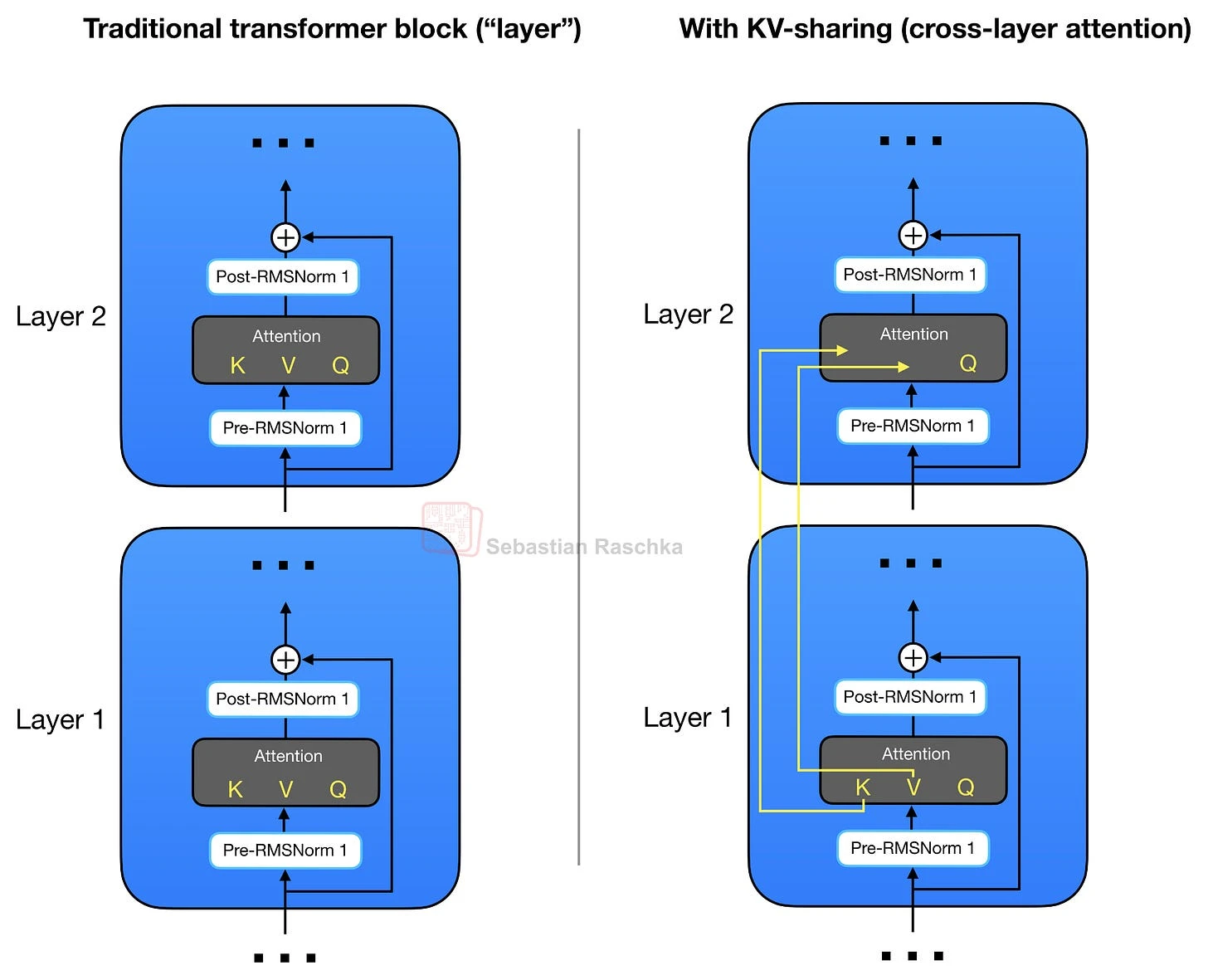
In Gemma 4, KV sharing is combined with GQA or MQA and sliding window attention — three of the techniques from this post in one model. The book’s simplified GPT example implements only the cross-layer KV-sharing part, so the code stays focused on the main mechanism.
The simplified rule it uses is:
- Early layers compute and cache their own K/V tensors.
- Later layers reuse the most recent K/V tensors from an earlier producing layer.
- All layers still compute their own query projections.
This reduces the number of K/V caches that grow with context length. The tradeoff is reduced model capacity, because some layers no longer get their own K/V projections.
My take: stacking GQA + MQA + SWA + cross-layer sharing in one model tells you these tricks are mostly orthogonal — each attacks a different axis of the same cache. Which also means the next efficiency jump probably won’t come from one clever idea, but from someone stacking a fourth.